Getting Started With DBT - Development Primer

In our previous guide DBT Cloud - Create a Project we learned how to build our first project in DBT, connect to our Snowflake database, and connect to our Azure DevOps repository. Now that we have our project and repo setup we are ready to begin development. This guide will walk you through the basics, a primer on how to get started working in DBT.

* All work we are doing is in the DBT cloud.

Navigating Your Project

In the top right corner of the DBT cloud interface you will see your organization name and a drop down list--this will contain a list of all projects in your organization. When you select a project, this will change the context of the Develop, Deploy, Environments, and Jobs options to the selected project. Before we can start modifying our project we first need to create our credentials for the target project. Any permissioned user in your DBT environment will still need to create credentials for the target project they want to work in before they can access the project through the Develop interface.

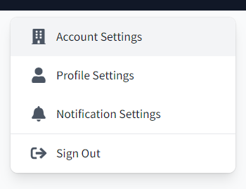
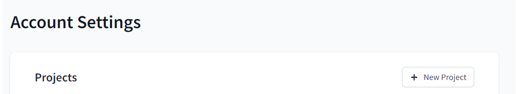
Click on the gear icon in the top right corner of the DBT cloud interface and select the Account Settings option. Once you are in Account Settings you will see other options to do things like create a project or set credentials. Since we already created our project in the previous guide, now we are ready to create our first set of development credentials for our project.

 In the Credentials section you should see a list of all projects in your environment.

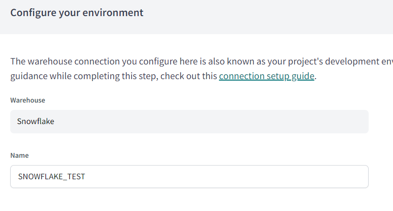
 Click the target environment and this will bring up options to establish your development credentials.

If your target database is Snowflake for example, then you should configure your Development Credentials with the credentials you access Snowflake with. So enter the username and password for your Snowflake login and for the schema, we want to specify a name that lets us know from where, who, and what project. In DBT, in your development environment,  when you materialize tables or views those objects are created in the schema you specify in your project development credentials. When you move in to production, these objects will materialize in the schema defined in your environment, more on that later.

I like to follow a naming pattern as such: <SOURCE_PERSON_PROJECT>. So let's say our project is named Accounting_Datamart, the schema I would enter is DBT_BHETT_ACCTMART. The system generating the object is DBT, BHETT is an abbreviated user name, and ACCTMART as an abbreviated project name. Once you start working across many projects this will start to make more sense--the goal here is to accurately track what assets you have created in DBT and what project they belong to. Once you are finished creating your development credentials there is one more step before we can start working in our project and that is to create the first environment. In the top navigation bar, click the Deploy dropdown and then select Environments.

On the Environments page click the Create Environment button.

For our first environment we are going to create a development environment.

Give your environment a name and select Development for the Environment Type. For DBT version I would always try to use the latest. Save that and we are now ready to start working in the project.  In the top navigation bar, click the Develop button.

Once the environment loads up you will see something that looks like the following.

Since we already created a relationship between DBT and DevOps when we built the project, all branching and merging is managed by DBT. When you click the Create branch button and create a development branch, DBT will create that in the remote repository and then check it out for you--all changes will be captured in this branch. When you are done with your development you can simply commit your changes in DBT and it will commit and sync them with your remote repository--DBT is acting as your git client here. You can also merge your development branch to main from DBT, but you should put in controls that prevent this behavior for the same reasons you prevent developers from merging to main anywhere else.

Notice all the folders and files in your file explorer, this is where you will build and organize the content for your project. The most important folder in your project is going to be your models folder, this is where you define all the SQL transforms for your data; how you organize this data will determine whether or not DBT is building views or physical tables--we will come back to.

First let's talk about the yml files. Yml files are configuration files that let you instruct behaviors and configurations in your project, models, tests, etc., and the most important of these at this point is your dbt_project.yml file. The project configuration file can be used for many different types of configurations as seen in the following link.

 https://docs.getdbt.com/reference/configs-and-properties

We are going to focus on some basic configurations for your project file. The project.yml file will already have some content when you open it, it will look something like this.

# Name your project! Project names should contain only lowercase characters
# and underscores. A good package name should reflect your organization's
# name or the intended use of these models
name: 'dbt_My_Project'
version: '1.0.0'
config-version: 2
# This setting configures which "profile" dbt uses for this project.
 profile: 'default'
# These configurations specify where dbt should look for different types of files.
# The `source-paths` config, for example, states that models in this project can be
# found in the "models/" directory. You probably won't need to change these!
model-paths: ["models"]
analysis-paths: ["analyses"]
test-paths: ["tests"]
seed-paths: ["seeds"]
macro-paths: ["macros"]
snapshot-paths: ["snapshots"]
target-path: "target"  # directory which will store compiled SQL files
clean-targets:         # directories to be removed by `dbt clean`
  - "target"
  - "dbt_packages"
# Configuring models
# Full documentation: https://docs.getdbt.com/docs/configuring-models
# In this example config, we tell dbt to build all models in the example/ directory
# as tables. These settings can be overridden in the individual model files
# using the `{{ config(...) }}` macro.
models:
   dbt_My_Project:
      datamart:
         materialized: table
      intermediate:
         materialized: view  

First you have the name of your project, you'll want to provide a name that accurately describes the project and you will then use this name in other configurations in your yml file. The next most important section is the paths section. This is what tells DBT where to look for certain types of files. I would leave this as-is for now and make sure you are creating content where DBT expects it (we will get in to this more later on). Finally, for your initial configuration you will want to start setting your materialization strategy. Setting materialization means instructing DBT what to do with your model definitions, which means creating tables or views.

In my file explorer I have created two folders under the model folder named datamart and intermediate.

For all SQL definitions in my intermediate folder I would like to have those rendered as a view, and for all SQL definitions in my datamart folder I would like those rendered as tables. In this configuration intermediate is my stage and datamart is the final dimensionalized object that reporting consumers will pull data from. I first write the SQL to transform the source data, denormalize, define custom attributes, create composite keys, etc. That is what we write to a view. Then we pull the data from that view and create references to the view and other views so that it creates a lineage for us and instructs DBT in what order things need to be built.

In the configuration file example above you will see the section named models. This is followed by the project name we assigned at the top of the project.yml file and then one entry for the datamart folder and another for the intermediate folder along with the materialization strategy of table or view. This is how you configure materialization for your project.

* Important note - proper indentation and formatting of the yml file is necessary in order for the file to be parsed correctly. Anytime you   are following a guide on configuring yml files, make sure you are following the exact formatting laid out in those guides.

Lets go ahead and create our first branch, add folders to our project, modify the project.yml file, and create the first SQL transform file.  Click the Create branch button and provide a name for the new branch.

In the models folder in your project File Explorer create two new folders named intermediate and datamart, make sure both of these reside one level under the models folder like shown in the previous image. Now we are ready to modify the project.yml file. Click the file and we are going to make a few changes. First, give you project a name in the configuration file, we are going to name ours "dbt_my_project".

name: 'dbt_my_project'
version: '1.0.0'
config-version: 2

Now we are going to define materialization for the new folders we created, add this section to your project.yml file and click the save button in the top right corner.

models:
   dbt_My_Project:
      datamart:
         materialized: table
      intermediate:
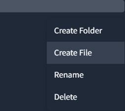
         materialized: view  

The last thing we need to do is to create our first SQL file. Highlight the intermediate folder and click the ellipses to the right and add new file.

Name this something like vw_stage_customer.sql or the name of a table in your target datastore, prefix with vw_ to communicate the materialization of the object, a view. Now write a simple query that returns a few rows and then click the save button in the top right of the screen.

Now we are going to create a file in the datamart folder, you can name this one something that better aligns with its role, something like dim_customer.sql, this one will be materialized as a table. For your query, write a select statement that calls all the columns you defined in your view and this brings us to the last and most important steps to get up to speed in DBT. Now we are going to add a reference and a surrogate key. First the ref function, more detail here.

 https://docs.getdbt.com/reference/dbt-jinja-functions/ref

Keep in mind, the ref function is a key feature in DBT. This is what allows you to build a lineage that is easy to understand and also instructs build order when your models are run. If you stick to the naming above, you can add your ref in your dim_customer.sql query like this.

 SELECT 
     CustomerId
    ,CustomerName
    ,StartDate
 FROM {{ref('vw_stage_customer')}}

For more details please refer to the DBT documentation, but this will get you the reference behavior that is central to the product. The last thing we want to do is to add a surrogate key, this is going to be a hash value key (not here to debate the merits of miisk vs hash keys). Before we can add the surrogate we first need to install the utilities that enable the surrogate key function. This is also another central feature to the DBT project, the ability to leverage libraries created by the community.

First thing we need to do is to install the dbt utility collection, instructions can be found here:

https://hub.getdbt.com/dbt-labs/dbt_utils/latest/

With that installed we are now ready to add the surrogate key function. Lets say we want to add a surrogate key based on the natural key CustomerId. This is how we would do that.

 SELECT 
    {{ dbt_utils.generate_surrogate_key(['CustomerId']) }} AS CustomerId_sk
    ,CustomerId
    ,CustomerName
    ,StartDate
 FROM {{ref('vw_stage_customer')}}

You can add more than a single field in the surrogate key generator. All fields will be separated automatically using a hyphen and that will be included in the hash key. So something like CustomerId, CustomerName would be rendered as CustomerId-CustomerName and that is the value that the hash is based on.

That should be enough to get you started in DBT. This is just a primer to get you up and running quickly, but there is still so much more to explore with the product. Advanced configurations, tests, and documentation are some of the other areas you will want to get up to speed in, but that will come in time as you use the product and have the need to implement those features.

DBT Cloud - Create a Project w/ Azure DevOps Repository

Projects in DBT are much like projects in any other IDE, think Visual Studio projects for example. A project will organize datastore connections, repository relationships, and all assets developed in that project such as DBT models, unit tests, configurations, etc. Before we can start working in DBT we first need to create a project.

This guide is for DBT Cloud, Snowflake, and Azure DevOps for your code repository. In the DBT documentation they suggest you would need the DBT enterprise licensing to connect to an DevOps repository, but that is only through HTTPS. We can still connect to a DevOps repository using SSH and we can do this at the standard licensing level of DBT.

This guide was written on 2023.02.10.

Project Configuration

First we need to navigate to your DBT cloud instance @ https://cloud.getdbt.com/

Make sure you are logged in to your account and once you are logged in, look to the top right hand corner of the DBT interface in your browser and you will see a blue gear, click that and then click the Account Settings option (the naming is not intuitive here, but the cloud interface will likely improve as the product matures).

On the Account Settings page, the first main section on this page will list all of the projects you have created. Click the New Project button to configure a new project, this will bring you to the project setup page.

The first option is to set the name of your project so give it a name that makes sense for the purpose or business system it serves. We have named our project MY_TEST_DBT_PROJECT for our example here. Once you have selected a name click the Continue button.

Next we want to choose our datastore (what DBT calls a warehouse), we are using Snowflake for this example. Select the target datastore and click next, this will take you to the configure your environment page.

The configure your environment page refers to the datastore configuration, this means everything we need to connect DBT to Snowflake. The warehouse will are configuring is Snowflake and it resides is Azure. Give the connection a name, we will name ours SNOWFLAKE_TEST.

As we move down to the Settings section, the first option is Account--this is your Snowflake account instance. If you have any firewalls enabled for your Snowflake instance, apply inbound filtering rules as needed. Configuring IP access is beyond the scope of this guide.

You can find your Snowflake account by pulling up your Snowflake instance in a browser. In the URL example below we have highlighted the part of the URL that describes the Account. We have to rearrange it to look like wc16274.east-us.azure and then enter that in the Account field.

"https:/app.snowflake.com/east-us.azure/wc16274/worksheets" is the URL, then your account will be wc16274.east-us.azure

Once we have entered the Account name, we are ready to move on to the Optional Settings section. While this says optional you will want to fill this out. For your Role, choose a security role you have defined in your Snowflake instance. In our example here we have a role named DATA_TRANSFORMER. For the Database, enter the target database you want to connect to in your Snowflake instance. Finally, for the Warehouse option, enter the appropriate compute warehouse you defined in Snowflake. I would leave the Session Keep Alive option unchecked. Your configuration should look something like the following.

The next section we need to configure is the Development Credentials section. This is where we configure the security credentials dbt will use to connect to the Snowflake instance for new development. Our Auth Method is Username & Password, but you can also use key pair if desired. Enter the Snowflake username and password for the account you want DBT to use to access your Snowflake instance. For the Schema option, this is the schema DBT will write to when you are working in your development environment. Depending our your team composition, how many people are working in DBT, you may want to tweak this to be more personalized. Here we are setting a generic schema of dbt_elt.

Make sure the user account and schema have already been setup in Snowflake. As for the Target Name and Threads options, I would leave these as the default for now. Here is what this section will look like.

Now you are ready to test your configuration. Click the Test Connection button at the bottom right of the page.

This will bring up a testing indicator. If you set this up correctly your testing should pass and we are ready to move on to the last section, Setup a Repository. This is where we are going to establish the relationship between our Azure DevOps repo and DBT. To do this we are going to use SSH.

Connecting to DevOps Repository

This section is a little more involved because we need to do a few things in Azure DevOps to get this working. Select the Git Clone option. DBT is asking for the SSH git URL which we will get from DevOps. Once we have the SSH git URL, DBT will create the public key that we will then load back to DevOps. This is how we build the relationship between the two systems.

Navigate to your target DevOps repository and click the Clone button in the top right of the landing page. There are two options, HTTPS and SSH, select SSH and then copy the URL DevOps generates.

Now that we have the target SSH URL we need to enter this in to DBT. Go back to the DBT configuration screen for the repository, make sure git clone is still selected, and then enter the SSH URL we copied from DevOps and click the Import button. DBT will generate an SSH key for us that will allow us to communicate with DevOps. We need to load this SSH key to Azure DevOps so,  copy the key and navigate back to your DevOps site.

In DevOps, in to top right corner, there is a person icon with a gear next to it. These are your personal settings and where you want to define the key. Click the icon and then select the option SSH public keys.

Click the New Key button, provide a name, and then paste the key you copied from DBT. When you are done click the Add button at the bottom of the page. You should see this in your list of public keys now in DevOps.

Go back to the DBT configuration page and click the Next button, this will complete the setup of your project.


How to Run DevOps CI/CD Pipelines for Paginated Reports That Use a VNet Gateway

This is a short guide on what you need to know to run DevOps pipelines on Power BI paginated reports that use a VNet gateway. This is written as of Aug 2022 while the VNet gateway feature is still in public preview. Hopefully, as this offering matures, we will see more options to make this work.

What Does Our Pipeline Do?

This guide does not include how to configure your pipeline, this guide is aimed at users trying to run their existing CI/CD pipelines for paginated Power BI reports that use a VNet gateway. The pipeline we are running does the following--deploys the target report to a development workspace, next it modifies the data source target and moves a copy in to a QA workspace. Eventually it will be moved to production.

What you need to know.

As of writing this, you cannot use an Azure Service Principal in your DevOps pipeline configuration, you must use a user principal that has MFA disabled. An Azure Service Principal cannot modify the embedded data source configuration of paginated reports that use a VNet gateway. The issue is that you cannot grant data source access to an Azure Service Principal at this time, only user principals. I imagine Microsoft will need to address this eventually.

Configuration Steps

Create a new user principal in AD to use for your CI/CD pipelines, we will need to permission this account in several places in Power BI.

Once you have the new account, log in to the Power BI service with an admin account and assign the new user principal to the VNet gateway and data sources used in your CI/CD pipeline.

First navigate to the VNet gateway - Options>Manage Gateways>Virtual network data gateways. Find the target gateway and click More actions>Manage users. Add the new user principal you created:

Next we are going to permission the new user principal to the target data sources. On that same page there is a tab for Data sources. We are going to assume you have already created a data source for each of your pipeline environments (dev, qa, prod, etc). We need to add our new user principal to each of these data sources. On the data source navigate to More actions>Manage users. Add the new user principal.

In Azure DevOps make sure the service connection is configured to use the new user principal we created. Go to DevOps and your target project. Click Project setting, under project settings look under the Pipeline group and click the Service connections option. You will see your service connections listed here.

Either modify the existing service connection that is using the Azure Service Principal or else create a new service connection. Either way we need to use the new user principal we created. Click on the target service connection and in the top right corner click Edit.

You can see there are two types of authentication methods here, one is the user principal and the other is the service principal. We want to select the username type and then complete the rest of the configuration as seen in the screenshot above.

Save the changes and you should be ready to run your pipeline. Double check all settings if you run in to errors. This has been validated as of Aug 2022.

Configure Paginated Power BI Reports to use a VNet Gateway

Part I - Data Source and the VNet Gateway

What is a VNet data gateway? According to Microsoft:

The virtual network (VNet) data gateway helps you to connect from Microsoft Cloud services to your Azure data services within a VNet without the need of an on-premises data gateway. The VNet data gateway securely communicates with the data source, executes queries, and transmits results back to the service.

The VNet gateway went into public preview in Aug 2022. For organizations that store data in the cloud (Azure data services) and want to expose that data to other cloud services (Power BI) without a public IP, they can do that now with a VNet gateway. In this example we are connecting Power BI reports in the service back to an Azure SQL Database via the VNet gateway.

Chances are the person reading this document will not be the person setting up the VNet gateway in Azure, to get with your systems and networking teams to get the VNet gateway setup before you do anything else.

Power BI Setup

Make sure you are a Power BI admin in the tenant. Log in to app.powerbi.com with your admin account. Click the gear in the topmost right corner, up around your account avatar, and click on Manage Gateways:

You should see three options on that page, Data Sources, On-premises data gateways, and Virtual network data gateways. We want to select the Virtual network data gateways. This is the VNet gateway setup by your cloud administrators. This is what will allow us to connect our Power BI datasets to our data sources in our Azure SQL database.

If you don't see anything in the virtual gateway list, make sure you turn on the option in the top right corner, it’s a toggle named Tenant administration for gateways:

If your admins configured the VNet gateway(s) and you have the correct permissions, you should now see your VNet gateway(s) listed here. Now we are going to navigate back to the list of data sources so we can add a new one that will use our gateway.

At the very top of the screen directly about the Data sources option, click on "New" to add a new data source. That will bring up the following window on the right of your screen:

Click the dropdown for the Gateway cluster name option, you should see a list of all available VNet gateways. Select the target VNet gateway--once your select a gateway a new option will appear in the window named Data source type. Give your data source a name and then select the correct data source type from the drop-down list. We are selecting SQL Server for our Azure SQL database.

Once you have selected the type, you will now see new fields to configure the connection. Add your server connection string, the same thing you use to connect to SQL from SSMS. We are using the basic authentication method; this will allow us to use a SQL Server account we have configured in our instance. It is preferred to use OAuth2. Once you have finished setting up the data source you should now see it listed on the page. Before you can use it, you need to assign permissions to the data source. Hover over the data source name and select Manage users.

Typically, you would want to setup a security group with all users who need access to this data source. Once you add the users you are now ready to use the data source. Next, we need to link this up to the paginated report.

Part II - Configure Paginated Reports to Use Data Source on VNet Gateway

Paginated reports (rdl) are a little different than your regular Power BI reports (pbix) in that paginated reports don't have a separate dataset; the dataset and the report are a single asset in Power BI.

Once you have published your paginated report from Power BI Report Builder app, go to the target workspace and find the report you published. On your report, click the three vertical dots for more options and then select Manage. This will take you to a screen where you can configure your data source via the gateway.

There is an implicit relationship detected by Power BI. It looks at the data source you configured in your report and will match that up with a gateway that uses that data source underlying connection. So if you setup you report using a dataset that you have not yet configured a data source for, it might give you problems.

Select the option to Use an On-premises or VNet data gateway. Expand the target gateway if you haven't already and under the Maps to option, select the data source we created in the part I of this guide. It should look something like this:

Once you map the data source you should now be able to run the report.

How to Implement Composite Security in Power BI - RLS for Paginated Report Visualizations

There are two types of reports in Power BI, the standard .pbix type which is native to the Power BI desktop and service, and then you have the paginated report type or .rdl, this type of report can only be created in Power BI Report Builder, a stand-alone tool for the desktop. You might recognize the .rdl extension from SSRS and that is because the Power BI Report Builder is just a lightweight version of SSRS. As great as Power BI is, we still have the need for paginated reports--pixel perfect reports intended for printing, rich data export options, or filtered, near real-time analysis of operational data. Microsoft continues to make moves to consolidate the SSRS features in to Power BI, but it is still a work in progress (as of 2023.02.03).

Microsoft introduced the paginated report visualization to Power BI in 2021 and it has been receiving more attention as of late, but the paginated integration with Power BI still has some glaring limitations and issues we assume will be worked out in the coming months. For a paginated report built on a Power BI dataset, it's not possible to call that paginated report from another Power BI report and pass down filters from the Power BI report to the paginated report. Well you can pass them down but they don't actually filter the data as you would expect. When you pass down filters to a paginated report that is built on a Power BI dataset it returns all data from the underlying dataset and then applies the filter. For very large datasets that just won't work.

 Problem Statement

Our report consumers want to be able to export data in different formats without some of the inherent limitations of exporting a single visualization in Power BI. Because our source data is so large, we need to be able to pass in filters to limit the amount of data we are returning to the client. We also want to preserve the Power BI user experience our report consumers are accustomed to with features like searchable parameters and a more presentable user interface.

The solution we present here is not ideal, but rather a workaround until Microsoft can address some of these issues.  You will see that even with the workaround, there are yet additional limitations to that as well, but this does solve a lot of our problems for now.

Paginated Reports in Power BI Desktop

Before we can call a paginated report using the paginated report visualization in Power BI, we first need to create a parameterized paginated report. We assume you all know how to do that already so we won't get in to the details of that. Once we have built the paginated report, we are now ready to call it from Power BI.

Open Power BI desktop and create a new report. Since the target paginated report we want to call accepts parameters, we first need to make sure we have a dataset defined in the Power BI report, from that dataset we will pull the filter parameters to pass down to the paginated report.

Because of the way Power BI processes filters, the filters you want to send to the paginated report, your filters must be related. This can present some challenges depending on how many filters your target report has since the greater number of filters means a larger cartesian product. Let me explain.

If the paginated report accepts 3 parameters - merchant, start date, and end date, then we need to pass those from the Power BI report and dataset. The same way we used to create datasets in SSRS with values that would populate a parameter in the report, we are doing the same thing here. First we create a table from a SQL query for all merchants and then we create a second table from SQL query for dates. We don't use a full dates table here because of the cartesian product we mentioned earlier (we will get in to the details of that next). Instead of a full range of dates we create the following:


SELECT 
   CONCAT(SUBSTRING(DATENAME(mm, MIN(CalendarDate)), 1, 3), '-', DATEPART(yy,MIN(CalendarDate))) AS DateLabel
  ,MIN(CalendarDate) AS StartDate 
  ,MAX(CalendarDate) AS EndDate
  ,ROW_NUMBER() OVER (ORDER BY MIN(CalendarDate) ASC) + 3 AS SortOrder -- plus the number of relative date attributes
  ,1 AS CommonKey
FROM dbo.DateDim
WHERE CalendarDate > DATEADD(DAY, -365, CAST(GETDATE() AS date)) AND CalendarDate <= CAST(GETDATE() AS date)
GROUP BY YearMonthName

UNION
SELECT 
  'Yesterday' AS DateLabel
  ,CAST(DATEADD(DAY, -1, GETDATE()) AS date) AS StartDate
  ,CAST(DATEADD(DAY, -1, GETDATE()) AS date) AS EndDate
  ,0 AS SortOrder
  ,1 AS CommonKey
UNION
SELECT 
  'Today' AS DateLabel
  ,CAST(GETDATE() AS date) AS StartDate
  ,CAST(GETDATE() AS date) AS EndDate
  ,1 AS SortOrder
  ,1 AS CommonKey
UNION
SELECT 
   'Last 7 Days' AS DateLabel
   ,CAST(DATEADD(DAY, -7, GETDATE()) AS date) AS StartDate
   ,CAST(GETDATE() AS date) AS EndDate
   ,2 AS SortOrder
   ,1 AS CommonKey
UNION
SELECT 
    'Last 30 Days' AS DateLabel
   ,CAST(DATEADD(DAY, -30, GETDATE()) AS date) AS StartDate
   ,CAST(GETDATE() AS date) AS EndDate
   ,3 AS SortOrder
   ,1 AS CommonKey
ORDER BY SortOrder, StartDate

This provides a good number of relative date slices representing the most common ways the data is interacted with. Now on to how we relate all this and why the number of records in each table matters.

Each table needs to be related in order for us to pass values from the different table down to the paginated report as input parameters. Because there is no relationship between merchants and dates, we will need to manufacture one with a common key. So in addition to the merchant and dates table we are also going to create a common key table. This common key or bridge table allows us to relate the otherwise unrelated tables. Create a common key attribute in each of your three tables and then create relationships between each of the three tables on that key. Because of the way these need to relate, you will need filtering in both directions and depending on how many parameters you have, many to many relationships even if there is only a single record in the bridge table. This is what we were referring to with the cartesian product, its why we want to limit the number of rows in a table used for parameter filtering.

Once you have set this up your report model will look something like this:

The way we setup this up is a requirement to be able to connect your parameters to the target paginated report. If you do not do this correctly you will receive errors when you try to define your filter parameters for the paginated report. 

Go back to your report view in your Power BI report and drag a few slicers to the report page. One slicer will list all merchants and the other will list the user friendly date labels you defined in your dates table. While you might think this is what gets passed to the paginated report its not actually. This is just filtering the data for the underlying parameter values we will map in the next step.

When working in Power BI desktop and you add the paginated report visualization to the canvas you will be presented with the following message:

Before we can connect to the target report we first need to define the report parameters in the Power BI report. When you have the paginated report visualization highlighted you will now see a parameters group in your Visualization tree where we can select the values we want to pass in as parameters to the paginated report. We have added our merchant number and start and end dates.

Once our parameters are defined make sure you are logged in to Power BI with a user account that has access to your organization's Power BI tenant. We are now ready to click the Connect to Report button that appears when we pulled the paginated report visualization on to the canvas. Click the connect to report button and we will be directed to a list of all paginated reports we have access to in our organization. This assumes we already have paginated reports deployed to our Power BI service, which we do, if not you'll want to create and publish one first. When you select a report from the target workspace we will then see an option to set the report parameters.

What is happening here is Power BI wants to know what values in the Power BI desktop report you want to pass in as parameters defined in the paginated report. We already defined our Power BI report parameters in a previous step, now we are ready to tie it all together. In the following image you can see we mapped the target parameter to the parameters we created in the Power BI report. If you set this up correctly you should be able to click the See Report button and the paginated report will be returned in the paginated visualization window.

Row Level Security (RLS)

 One of the nice features of using this pattern is we can apply RLS to the merchant table the same way we would on any other table in a Power BI report model. We can might use the USERNAME() or CUSTOMDATA() functions to filter the merchant table down to just what the report user needs to see. We have a security modifier in our merchant table query we can use to set the correct filter context based on the current user. The difficult part of building this pattern has less to do with the RLS piece and more to do with the constraints around pass through filtering for a paginated report visualization.

 In addition to RLS security the paginated report can have another layer of security baked in to the code for its underlying datasets, the same way you would have set it up for SSRS reports in the past. In SSRS there is a built-in field for the current user ([&UserID]) and you can use this to filter your report by joining to a dataset in your database that has permissions defined for the different users, a common pattern for this type of report.

 So between RLS in your Power BI calling report, data filtering on UserId in your paginated report, you can be sure that users only have access to the data they are supposed to see.

How to Prevent the Deletion of Datasets in Power BI

Note - This guide is being published in Oct. 2020. This month Microsoft began rolling out the "New Look" to the Power BI service. We have enabled the new look and the features underlying so any screenshots in our guide are based on the new look. Also to note, we are using SSAS tabular with a data gateway and a live connection from the Power BI service.

Update May 2023 - As of May 2023 the protected dataset is still the best approach to prevent the deletion of datasets (and associated reports) in your Power BI tenant. Store your datasets in a workspace that only admins have access to. Keep all master reports in your GIT repository. Share the protected dataset from the admin workspace to user groups in your organization. Hard to believe this is still an issue, but it is.

Overview

Datasets are what we use to build reports in the Power BI service. A dataset will reference a data source that has been configured in the Power BI service. We are using SSAS Tabular to build models that can be consumed by Power BI, we publish these models and then access them through a data gateway. We create the data sources on the data gateways in the Power BI Service and then link the data sets to the data sources.

All reports you build in the Power BI service are going to reference a dataset. If a single dataset has 100 reports built off of that data and somebody comes in an accidentally deletes that dataset, all the reports that are tied to that dataset are also deleted. Power BI is a self-service product and you want your teams to be able to build their own reports. In order for teams of a Power BI workspace to build their own reports you need to grant those users contributor permissions on their workspace. This permission also allows those users the ability to delete datasets and that is where you can run in to trouble.

For some reason Microsoft has not done a great job with options to protect content in Power BI. There is no concept as a recycle bin in the Power BI service, when it's gone it's gone. The security roles for workspaces are too broad, the main roles are admin, contributor, and viewer (we'll get more in to this in a minute) and most users will be in the contributor role if you want them to create their own reports (we do). The contributor role is over-permissioned unfortunately so we have to take extra steps to protect our content in Power BI.

That is the purpose of this guide, to you walk you through steps on how to protect content in the Power BI service and reduce the risk of a dataset (and all of the content that depends on it) from being deleted while at the same time enabling your teams to use self-service reporting and workspace management.

Dataset Basics

  • Datasets depend on data sources. We can define a data source on a data gateway but to create a dataset, we first need to create a report in the Power Bi desktop. In our environment our Power BI desktop report will use a live connection to an SSAS Tabular database/model. When we publish this report to the Power BI service it will create a dataset. We link the dataset to the data source.

  • When you delete a dataset in a workspace, all reports that are built from that dataset in that same workspace will be deleted along with it. If a report was created in another workspace that referenced the deleted dataset, that report will become orphaned and no longer work.

  • Datasets are based on GUIDs and not names. If you delete a dataset and try to republish it again with the same name, as far as Power BI is concerned that is a new dataset and no existing content can be linked to it. Since datasets are based on GUIDs and not names, it is possible to have more than one dataset with the same name so this could cause some confusion in a workspace.

  • A dataset inherits permissions from the workspace it resides in, but it can also be granted additional permissions beyond the workspace permissions by modifying the dataset permissions (we will explain this below).

Workspace Configuration

In order to protect our Power BI datasets we need to store them in a workspace that only your BI developers have access to. From there we will grant build permissions to users on the datasets we publish in this workspace but they won't have access to delete that dataset. Using this along with version control (DevOps, BitBucket, etc.) is the best way to secure and protect content in your environment.

Note - what we are doing here assumes you and your users are using the Power BI environment in the Professional or Premium capacity. You will need this type of licensing to share content across the organization.

In the Power BI Service, create a new workspace named BI Admin. For the members, start by granting admin rights to your BI Developer admin(s). These are the people who will publish, modify, and maintain all the content in this workspace. In the screen shot below you can see we created the new workspace and permissioned myself as admin to the workspace, but there is no content in the workspace yet. While we are at we are also going to add a single user who only has view permissions in the workspace. This is the user we will delegate build permissions to on the dataset.

PBI_Dataset1.jpg

Publish Dataset

Now we are ready to publish our first dataset to the secure workspace.  Remember, we are using an SSAS tabular model with a live connection, your environment might be different but the securing process is still the same.

Open Power BI desktop and make a connection to your data source, for us that is an SSAS tabular model.

PBI_Dataset2.jpg

When you connect to the SSAS tabular model your will see all the tables in the model populate in the report.

PBI_Dataset3.jpg

On the report canvas there is no need to create a visualization, what you should do instead is to make a note about the report and the dataset, something that tells you what it is and what team it is for. For example, if this dataset is for the "Product Team" I might add something like you see in the screen shot below.

PBI_Dataset4.jpg

When you publish your first report for a particular dataset to the Power BI service it will also publish the dataset that report is connected to. In the case of our report here it is connected to the SSAS tabular model for the Adventure Works database. It's important to keep in mind that the dataset in the Power BI service will have the same name as the report it references. You do not want to rename the dataset after it is published, instead give your template report a name you want reflected in the dataset, something like "Product Support Dataset".

Now we are ready to publish this to the Power BI service. Click on the Publish button on the home tab, select the target workspace, in this case the BI Admin workspace, and click the Select button.

PBI_Dataset5.jpg

You will see the following message when the report and dataset have been published.

PBI_Dataset6.jpg

Now let's open up the Power BI workspace we created earlier, you should now see your report and your dataset.

PBI_Dataset7.jpg

I understand the naming around the report doesn't make much sense, but we don't want to rename the dataset after it is published so we give the report a name that best suits the dataset. After we have published the dataset next we need to link it to a data source. Click on the Manage Gateway option in the settings gear. When you are in the Gateway settings, click Add a Data Source and add the model of the SSAS tabular model your dataset is based on. You will need all the details of the SSAS server you are connecting to, this also assumes you already have the data gateway up and running.

PBI_Dataset8.jpg

Once the data source has been added we can go back to settings of the dataset. Expand the Gateway connection section and for the target database, select the data source you just added in the previous step. As you can see in the image below, we named the target data source AdventureWorks.

PBI_Dataset9.jpg

If you recall earlier, we setup a user on the workspace that has only view permissions. That user is a member of the Product Support team and wants to use the new dataset we just published to build reports from. We want to make sure the user can't delete the underlying dataset thus deleting any reports tied to that dataset. So what we are going to do is give the user build permissions on the dataset directly, this will allow them to build reports off of the dataset but will not let them modify the dataset. If this user was a contributor to the workspace they would be able to delete the dataset, that is what we are trying to prevent.

By default the dataset will inherit permissions from the workspace, but we can grant additional permissions on the dataset. Click on the Manage Permissions option of the dataset.

PBI_Dataset10.jpg

Now we can grant the build permission to our view only user, this will allow that user to select this dataset and build reports from it while working in their own workspace. It's basically sharing the dataset without elevating the users rights to the dataset beyond exactly what they need.

PBI_Dataset11.jpg

If our user Kevin wants to build a report from this new dataset, in Kevin's team workspace he can click New>Report. From there he can view all datasets he is permissioned to and can select the Product Support dataset we just published and granted build permissions on.

PBI_Dataset12.jpg

Now we need to select the Product Support dataset and click create. This will effectively create a linked reference to the dataset allowing the user to create a new report in their workspace.

PBI_Dataset13.jpg

When they save the report they won't even see the dataset in their workspace much less be able to delete the master copy of it. This is how we ensure that our users have permissions to create and modify their own content without running the risk of errantly deleting a dataset that then wipes out reports for the rest of the team.

Also, now when we want to add changes to the underlying data model in SSAS all we have to do is update the model, refresh the report in Power BI desktop, and republish the report back to the Power BI service. This will preserve all connections from reports to the dataset while also giving those reports access to the new assets published to the SSAS model.

Salesforce Data Integration Primer - ETL and SSIS

If you are working with Salesforce, especially if you are building out your first instance, you will likely need to populate Salesforce with at least some of your existing data. That could be from a legacy CRM or from other business systems you wish to enrich your Salesforce data with. Once your Salesforce instance is loaded and launched to production you will likely have ongoing integration needs where you will be sending data to Salesforce from on-prem databases and loading those same databases from Salesforce. While Salesforce does offer some decent reporting capabilities it is likely you'll want to bring your Salesforce data down to your ODS or Data Warehouse where you can join it with the rest of your business data to gain the most meaningful insights.

While there are other ways you can integrate data to and from Salesforce, we are focusing on the Business Intelligence wheelhouse. For example, if you wanted to cascade data in real-time from other source systems to Salesforce, you could build that out in custom development. For different reason you may not need that kind of custom solution and a scheduled, incremental data load would suffice.

Some Considerations

Here are some considerations you will likely wrestle with as you get started and some good to know facts before you tackle your first Salesforce integration project. This is a wide-angle view--we will go into more detail later in this guide. 

  • The different types of integration tools we can use to load and extract data from Salesforce.

  • Data integration is performed by accessing Salesforce APIs. Salesforce API endpoints have a standard and bulk processing mode. Use the bulk API to load large amounts of data without consuming too many API calls. Use the standard API to process small batches and properly report on errors.

  • You have a limited number of APIs you can consume each day and this is dependent upon how many users you have licensed in Salesforce.

  • There is a canned report in Salesforce that will tell you how many APIs each user has consumed each day for the last seven days. This is helpful to track how many APIs your data integration process is consuming.

  • When updating data in Salesforce you must use the Salesforce Internal Id (Id). If you want to upsert (insert/update) data to a table in Salesforce you need to create an External Id that is unique in the target table.

  • The lookup data type in Salesforce can only reference another field using the Salesforce Internal Id (Id). You cannot use an External Id or other field.

  • Get familiar with the way Person is modeled in Salesforce. You can have the Individual model or the Person Account model. How Person is modeled will affect how you relate data in Salesforce.

  • In the person account model, contact records are stored in the account table as well as the contact table. In order to relate account contacts to their parent account in the account table, you need to use the AccountContactRelation table in Salesforce.

  • Get familiar with the Setup section in the Salesforce application, this is where you can learn a lot about your environment. Included here are things like the object model in a nice customizable visualization, bulk data load tracking and history, error logs, and feature settings. Make sure you have access to Setup in Salesforce.

Integration Tools

As you start down the road of data integration with Salesforce its good to know what tools you have available to you. Below is an overview of some of the more common tooling for data integration with Salesforce.

Data Loader - The first and most common data integration tool you will hear about when getting started with Salesforce is the Salesforce Data Loader. This is a free tool Salesforce provides that allows users to load files to Salesforce and also export Salesforce data as a file. While you cannot automate work through the Data Loader tool, I would probably install it anyway and get familiar with it. There is a good chance that somebody in your organization will use Data Loader at some point so it's good to know what it can do.

SSIS Integration - Out of the box, SQL Server Integration Services (SSIS) does not support connectivity to Salesforce but there are a number of companies providing tools that will give you Salesforce connectivity inside of SSIS. Most add-in packages for Salesforce include Salesforce data connectors, Source, Destination, and Lookup components which provide all the integration points you will need for your project. Products we have tested and like are SentryOne SSIS Task Factory, CozyRoc SSIS, Devart Data Flow Components, and ZappySys SSIS Components. The cost of these tools are relatively cheap, $300 - $2000 for a server license. The client tools are free though so you can use and test any of these on your workstation. Of the add-ins mentioned above we liked the SentryOne SSIS Task Factory best.

Because of its ubiquity, community support, free license with SQL Server, and ease of use, SSIS can be a great option. Coupled with some cheap Salesforce add-ins, the cost of integration tooling barely registers a blip on the technology budget radar. If you don't already have Microsoft SQL server in your organization, you might find better options out there.

Apex - If you don't have a data integration or BI developer on staff you can always turn to your app devs for your integration needs. Apex is an object-oriented programming language used exclusively for Salesforce. Apex allows you to execute flow and transaction control statements in Salesforce in conjunction with calls to the API. There are some things, like complex workflows that might require some custom development with your app dev team, but day to day integration tasks are probably better kept with your BI and data teams.

iPaaS - Integration Platform as a Service (iPaaS) is new to a lot of organizations but if you already make use of one--Boomi, Mulesoft, Jitterbit, et al, then you already know what it can do. Without getting too deep in what iPaaS is and what it can do for you, I will say that it can be a great tool for building data integration workflows with Salesforce as well as building complex data integration workflows across multiple disparate systems. Out of the box iPaaS tools have everything you need to integrate with Salesforce. iPaaS isn't cheap though, so if your only business use case is Salesforce integration there are probably better options out there.

Skyvia - As a standalone integration tool, Skyvia can help you will all integrations related to Salesforce. Skyvia is produced by Devart a company that also produces the Devart SSIS components for SSIS. I don't have a lot of experience with this tool so I don't have much to say about it. All I know is that this company is based out of Ukraine and so reaching them during business hours in the west can be a challenge. Aside from that, the feedback on this product is pretty good and worth a look if it makes sense for your environment. Pricing is based on number of records processed and starts at $4800 for 10 million records processed per month.

Capstorm - Is a Salesforce data backup and recovery tool that can also be used to replicate data in and out of Salesforce. I don't think you would use this in most common data integration scenarios, but it does have its uses. Worth a look if you also plan on implementing a robust backup solution--it is a leader in that space.

Now that we know what Salesforce integration options are available to us, let's move on to some of the more nuanced discussions around getting data in and out of Salesforce.

Data Integration and Salesforce APIs

The way you integrate data with Salesforce is through one of the Salesforce APIs. You will use either the standard API (REST or SOAP) or the bulk API and it's important you understand the difference between them. It doesn't matter what integration tooling you use, you still connect to the same APIs and you still have the same constraints of each of those. When thinking about common, schedule-based data integration processes you need to choose how you will connect to Salesforce, with the standard or bulk API.

The reason why this is so important is because of the way Salesforce licenses API calls to its system. For each user license you have in Salesforce you are allowed 1000 API calls per day. That includes the API calls those users are making through the Salesforce application. If you are pushing the limits of your daily API cap, the standard API might not be the way to go for your organization. The standard APIs are restricted to much smaller batch sizes compared to the bulk API resulting in higher API counts per data integration operation. The bulk API allows for much larger batch sizes, 5k + per batch. This is an important consideration when you are getting in to data integration with Salesforce and guess what, those API counts are not the only thing you need to be concerned with when using the different APIs.

There is another key difference between these types of APIs that you need to be aware of. When working with the standard API you are basically getting row by row feedback for your data integration operations so if a record fails and the job fails with it, you get that feedback right away whether that is in Data Loader, SSIS, Apex, or iPaaS. The bulk API is different though, instead of going row by row the bulk API produces a large file per batch and then submits that to Salesforce for processing. That means that once you have submitted that batch through the Bulk API failures will not be reported back to the application you submitted them with. In Salesforce there is a section where you can see the status of your bulk API jobs, they can be found here: Setup>Platform Tools>Environments>Jobs>Bulk Data Load Jobs. This is important to note because data loads using the bulk API can feel like a black box unless you know where to look for status on the load you submitted. This is also where you can find errors related to your data loads so you know what needs to be corrected.

It might make more sense to use the bulk API for large loads and use the standard for everything else. If you can build a good incremental workflow this should set you up to use the standard API most of the time. It might just be for those initial loads that you would use the bulk API. Your mileage may vary but these are things you want to have on your radar. Also, don't forget to track down the canned Salesforce report on API usage. This will show you the API usage by user by day for the last seven days.

DML Operations in Salesforce

When it comes time to actually update the data in Salesforce there are several rules you need to follow. There are different DML operations you can access in Salesforce such as insert, update, delete, upsert, and merge. One thing to note about merge, this is not the same as the merge in SQL Server so if you are looking to update/insert in the same operation you can use the upsert option in Salesforce. There are some other nuances about the different DML types you should know.

If you are updating data in Salesforce you need to do that on a Salesforce Internal Id. A Salesforce internal Id is what Salesforce uses to uniquely identify a row in a table in their database-- this as an auto generated identity column, each time a row is created a new Salesforce internal Id is created to represent uniqueness in the table. The only way you can update (not upsert) a Salesforce table is by using this Salesforce internal Id, you cannot update data without it. You will probably end up with some kind of workflow that brings Salesforce data in to your local environment, uses an External Id to join to you other source data, and then uses the Salesforce Internal Id you brought down to do an update, Or…

If you need to upsert (update/insert) data you can't do this on the Salesforce internal Id, for this you will need a Salesforce external Id. A Salesforce external Id is a way for your business to uniquely identify a row in a Salesforce table using a business key, a value that has meaning to the business. You will select and or create a field in the desired table in Salesforce and designate that field an ExternalId, and while it is not required I would also recommend setting the value as unique because you can't upsert on the table if the value is not unique. Once you have the unique ExternalId configured for your target table you can start upserting to the table.

Establishing Data Relations in Salesforce

Loading data is only the beginning, you need to make sure all the data you are loading is properly relating across the Salesforce instance. One of the areas you might get hung up on early is the Person model in Salesforce. Salesforce has different ways you can model Person - the Individual and the Person Account model. I would encourage you to go out and read more about this, Salesforce has some good documentation around it. What I would like to talk about here is the Person Account model, how that works and how you build relationships with the Person Account model.

In the Person Account model, contacts are stored in both the Account table as well as the Contact table. When you load an account contact to the account table, a contact record is also created in the Contact table in Salesforce automatically. In the Account table you can have many different types of account so let's assume we are working with two types for this example, an Account Household and Account Household Contact (members of the household). Once we load both the Account Household and the Household Contact next we need to tell Salesforce they are related and to do that we need to use the AccountContactRelation table in Salesforce. The AccountContactRelation table is a bridge table/junction object in Salesforce that connects a contact record to an account record using the Salesforce Internal Ids of both the account and the contact. This is the primary way you will relate contacts and accounts in Salesforce in the Person Account model.

Other ways you can relate data in Salesforce is to create or make use of lookup fields. A lookup field is a data type in Salesforce that expects a Salesforce Internal Id on which to lookup/relate the value for. Lookup fields are only compatible with Salesforce Internal Ids, they will not work with an External Id or other field types. Imagine you have an Account type of Registered Investment Advisor (RIA) and you have Advisors who work for this RIA. If you want to relate the Advisor to the RIA you might have a lookup field named Advisor in the Account table that is a lookup data type. This uses the Salesforce Internal Id for the Advisor which provides a lookup for the Advisor record in the RIA record thus building a kind of relationship between the two record types.

You can also build your own junction objects for many-to-many relationships but for one-to-many you can use the lookup fields.

Setup and Troubleshooting

Inevitably you are going to run in to issues during your Salesforce integration project so you need to know where to look. The best resource is in the Setup interface in Salesforce which can be reached by clicking the gear in the top right corner of your Salesforce application and clicking the Setup option. Make sure you have the correct permissions to see this. Once you are in the Setup section you should have access to the Following:

Schema Builder - This is where you can find the relational model (object model) for your Salesforce instance. This has a nice customizable interface that will give you greater insight in to the database relations in Salesforce. Can be found here:

o    Setup>Platform Tools> Objects and Fields>Schema Builder

Object Manager - This is where you can view the fields and attributes configured for Salesforce tables (objects). This can be found here:

o    Setup>Platform Tools> Objects and Fields>Object Manager

Bulk Data Load Jobs - If you are running bulk API jobs you will want to know more about the execution of those jobs and to do that you will need to go to the Setup section that shows active jobs and a history of all jobs run including an errors in those jobs. These can be found here:

o    Setup>Platform Tools>Environments>Jobs>Bulk Data Load Jobs

API Usage Report  - This is something you will need to keep an eye on. Here are instructions for viewing or creating this report: https://help.salesforce.com/articleView?id=000326126&type=1&mode=1

Conclusion

This should provide a good primer to get you up to speed with data integration in Salesforce. Once you know all the rules and how to make it work, it really is quite easy.

Remove Empty Row from CSV File Using PowerShell in SSIS

When you export data to a flat file destination in SSIS you end up with an empty row at the end of the file. This is by design, because each row requires a CR LF. That last row of data still has a carriage return at the end of it thus the blank row that follows.

Finding a solution to this problem is not straightforward and that is likely due to the fact this is not really a problem, but not everyone will agree with that opinion. If you have been Googling you probably stumbled upon the conditional split solution, but that only works if you are starting from a csv that has the trailing blank row and you are writing that data to some place other than a flat file destination. We want to remove the empty row after we write to the flat file destination.

If you are not a C# developer or a VB developer (nobody should be one of these actually), then you might struggle with the script task in SSIS. Instead of that we are going to invoke a process, PowerShell.exe. Here are the steps you will need to follow:

  • Make sure PowerShell is installed/enabled on the server that the package runs on.

  • On the server where your SSIS package is executed, we need to create the PowerShell script to remove the blank row (below). Replace the value in the $textFile variable to your target file. Save the script in a directory where the SSIS service account can execute the file and modify the file, etc. Save the file as PS_RemoveBlankRow.ps1 or whatever you like.

$textFile = 'C:\YourFileShare\YourTargetFile.csv'
[System.IO.File]::WriteAllText($textFile, [System.IO.File]::ReadAllText($textFile) -replace '[\r\n]+$')
  • Before you can remove the empty row from your file you first need to save the file to its final destination. So work through all the steps in your SSIS package to get your data to the desired flat file.

  • Now we are ready to clean the file. In the control flow tab of your package add an Execute Process Task. Click on the Process tab, in the Executable option type PowerShell.exe, this will invoke PowerShell. In the arguments type the following (below). The –F option is for file, then you are entering the directory and file of the PS file we created in the second step. You can leave the rest of the settings to their defaults.

-F C:\MyFileShare\PS_RemoveBlankRow.ps1

  • You might have to grant an exception on executing this script file if you have some kind of AV that blocks it. Depends on your environment.

There you go, a simple way to remove the trailing empty row in a CSV.

Connect to Azure CosmosDB with MongoDB API from Studio 3T for Mongo

Let's assume you've created a CosmosDB database with MongoDB API in Azure and you would like to connect to it using Studio 3T for MongoDB. Follow these steps to connect.

In Studio 3T, click the Connect button and then click New Connection—this will open the new connection dialog box. At this point you will also want to connect to Azure and open your CosmosDB database.

img1.jpg

You need to get the connection details for the 3T dialog from your CosmosDB database configuration. In Azure, click on the Azure Cosmos DB link, and then click the target database, this should bring you to the database overview. You will see a tree view of options, under settings, click on the Connection String link, this is where you will get all the details to connect to your CosmoDB database.

In the 3T connection dialog, select Direct Connection for the Connection Type, for the Server you will use the HOST name from Azure. CosmoDB does not use the default MongoDB port so make sure you use the correct port from Azure. Once you have finished adding your server name and port you can click on the Authentication tab.

img2.jpg

For the Authentication Mode, select the Basic MongoDB type. For the User name, copy the USERNAME from Azure. For the Password, copy the PRIMARY PASSWORD from Azure. Authentication DB is admin and you can optionally configure the "Manually list visible databases" option as seen in the screen shot above. Now we are ready to move on to the SSL tab.

img3.jpg

Check the box to "Use SSL protocol to connect" and then click the "Accept server SSL certificates trusted by the operating system" option.

Save the connection and then click connect.

Default Schema and Schema Scope in Stored Procedures

When working in SQL server, if you call an object--EXEC, SELECT FROM, etc, you can do so without specifying a schema and it will default to dbo (unless you have assigned a different default schema to that user, though it is more common not to). What happens if you have a procedure in, let's say, a dev schema and you are calling tables from both the dev and dbo schemas inside it? If you are including the schema names in your query <SchemaName.TableName> then everything will work as expected, but what happens if you exclude the schema from a table you are calling in hopes that it will return dbo? That depends on where the table exists, in dev, dbo, or both and what schema the calling object belongs to. 

I wanted to put together a script that explains the behavior of default schema and schema scope in stored procedures. Let's walk through the following script for a more meaningful explanation.

--======================================================
-- Default Schema and Schema Scope in Stored Procedures 
--======================================================

-- Create a dev schema if you don't have one already

CREATE SCHEMA [dev] AUTHORIZATION [dbo];
GO

--DROP TABLE IF EXISTS dbo.ordertest;
--DROP TABLE IF EXISTS dev.ordertest;

-- Create a table in the dbo schema

CREATE TABLE dbo.ordertest (
ID smallint,
Targets varchar(20) );

INSERT INTO dbo.ordertest
SELECT 1, 'dbo';

-- Create the same table, this time in the dev schema

CREATE TABLE dev.ordertest (
ID smallint,
Targets varchar(20) );

INSERT INTO dev.ordertest
SELECT 1, 'dev';
GO

-- Notice we populate the dbo.ordertest with the targets value of dbo and the the dev.ordertest with dev

-- Now we need to create a stored procedure in the dev schema. We create this without specifying the schema in our SELECT table. 

CREATE PROCEDURE dev.TestSchema AS
    SET NOCOUNT ON

        BEGIN
        SELECT * FROM ordertest -- No schema specified here
        END;
GO

-- Now lets do a simple query against ordertest without specifying a schema

SELECT * FROM ordertest

-- The result is dbo, because dbo is the default schema in SQL

-- This time we specify the dev schema and get the value from our dev table

SELECT * FROM dev.ordertest

-- What happenes when we call our stored procedure in dev, which performs a SELECT against the table without a schema?

EXEC dev.TestSchema;

-- Returns dev, because the scope of the stored procedure is the dev schema, so it assumes an undefined schema is the same as the object calling it.

So if we have two tables of the same name in a SQL database that belong to two different schemas, if you call one of those in a SELECT without specifying the schema you will get the table in the dbo schema because that is default schema in SQL. If you write that same SELECT without specifying a schema and drop it in a stored procedure that belongs to the dev schema, when you execute that stored procedure it will return the results from the dev table because dev is the schema scope for that procedure. This can be confusing if you are expecting the result from dbo since that is the behavior you are used to. Now what happens if we delete the table in dev and call the procedure again?

-- What happenes if we delete the dev table and then run the procedure again?

DROP TABLE IF EXISTS dev.ordertest;

EXEC dev.TestSchema;

-- Now it returns dbo.

Now the query returns the result from dbo because the table no longer exists in the dev schema (the scope of the stored procedure) so it once again defaults to dbo. One more reason to always include schema names in all of our queries, that way you never run in to the situation we have illustrated here.


Upgrade SQL Server SSRS to Power BI Report Server

Wanted to make a quick guide on upgrading SSRS Report Server to Power BI Report Server. This is an in-place upgrade, we will replace the existing SSRS Report Server with Power BI. These are the upgrade steps for SQL 2016--I can't say how different this process is on an older version though I can't image much. Power BI Report Server is a stand alone product now. Here are the steps you will need to follow.

  • Take a full backup of your ReportServer and ReportServerTempDB databases
  • Backup the SSRS Encryption Key and make sure you save the password you used to back it up.
  • Stop the SSRS Report Server service
  • Detach the ReportServer and ReportServerTempDB databases (we want these in case we need to roll back, your backups would work also, up to you).
  • Restore the ReportServer and ReportServerTempDB databases you backed up, keep the same database names but give them new physical file names, for example, PowerBIReportServer.mdf.
  • Install the PowerBI Report Server
  • Configure the PowerBI Report Server.
    • Start the service
    • When you configure the http reservations, it will override the existing SSRS Report Server reservations. That is fine and what you want; you will see a warning when this happens, you can ignore it. If you had to roll back, when you uninstall the PowerBI Report Server it would release those reservations back to SSRS Report Manager.
    • Point the service at the existing databases you just restored. Important note here: because we are effectively restoring SSRS Reporting database to the PowerBI Report Server, it's important that you don't change the names of these databases. Your SSRS report subscriptions will be looking for the original name of the databases, if this is changed your subscriptions will not work.
    • Make sure you configure your email setting on the new server. If you fail to do this you will get an error when you try to open existing subscriptions on the server, because it is expecting those mail settings.
  • Once you have finished configuring the server, restore the SSRS encryption key you backed up. This will restart the service at which point the upgrade is complete.

Not a lot to it, but there were a few things not mentioned in the Microsoft guide which is why I wanted to create this here. Keeping the database names the same and also the issue with email configuration and subscriptions. It's a pretty simple upgrade and the new PowerBI Report Server is a nice addition to the Microsoft BI stack.

Current Year, Previous Year, The Missing Dates Problem, and LAG

When working with data that has date gaps, we need to have different ways of filling in the missing dates. This could be something like previous revenue where you want to see what a customer purchased last year but they don't have a sale in the current year. Or maybe you want to carry a value forward over a certain period where you are missing dates, like a rate value over a holiday. I want to go over several different scenarios and ways to solve these problems. We will look at issues with LAG when dealing with missing years, single missing year vs. multiple missing years, and the different methods we can use to fill in the gaps.

The first problem we will look at is the previous year issue. We want to see revenue totals and previous years revenue totals for customers even if they don't have a sale in the current year. For simplicity, our sample data only contains a single customer, but the solutions here have proved performant across larger data sets. We have the customer, sales year, trimester, and revenue. You will see that the customer has no sales in 2013 or 2017 so we can address the missing years. Sales are mixed across different trimesters in different years to provide all the different previous year scenarios.

DROP TABLE IF EXISTS #Sales;

CREATE TABLE #Sales (
     CustomerNumber int
    ,SaleYear int
    ,Trimester int
    ,Revenue decimal(7,2) );

INSERT INTO #Sales
SELECT 333, 2012, 1, 25.00 UNION ALL SELECT 333, 2012, 1, 44.00 UNION ALL SELECT 333, 2012, 3, 18.00 UNION ALL SELECT 333, 2012, 3, 12.00 UNION ALL
SELECT 333, 2014, 1, 18.00 UNION ALL SELECT 333, 2014, 1, 24.00 UNION ALL SELECT 333, 2014, 3, 15.00 UNION ALL SELECT 333, 2014, 3, 24.00 UNION ALL
SELECT 333, 2015, 1, 56.00 UNION ALL SELECT 333, 2015, 2, 6.00  UNION ALL SELECT 333, 2015, 3, 31.00 UNION ALL
SELECT 333, 2016, 1, 43.00 UNION ALL SELECT 333, 2016, 1, 11.00 UNION ALL SELECT 333, 2016, 2, 36.00 UNION ALL SELECT 333, 2016, 3, 31.00 UNION ALL
SELECT 333, 2018, 1, 29.00 UNION ALL SELECT 333, 2018, 1, 33.00 UNION ALL SELECT 333, 2018, 2, 17.00 UNION ALL SELECT 333, 2018, 3, 16.00 ;

In our first example we look at how to get previous year, year over year, without addressing the missing year using the self-join method. Because our customer has multiple sales in the same year and trimester we summarize the data in a CTE before doing our self-join for previous year.

-- Get total revenue by Customer, SaleYear, and Trimester

WITH CTE AS (
    SELECT 
         CustomerNumber
        ,SaleYear
        ,Trimester
        ,SUM(Revenue) AS Revenue
    FROM #Sales 
    GROUP BY CustomerNumber, SaleYear, Trimester )

-- Then use self join to get revenue for previous year

SELECT 
     c.CustomerNumber
    ,c.SaleYear
    ,c.Trimester
    ,c.Revenue AS CurrentRevenue
    ,ISNULL(p.Revenue, 0) AS PreviousRevenue
FROM CTE c
LEFT JOIN CTE p ON c.CustomerNumber = p.CustomerNumber AND c.SaleYear = p.SaleYear + 1 AND c.Trimester = p.Trimester
ORDER BY c.Trimester, c.SaleYear;

In the query above we are self-joining the CTE; if we didn't have to summarize the data we could exclude the CTE and just self join to the table (personal note, I find CTE's more readable for queries like this). The key here is in the join condition c.SaleYear = p.SaleYear + 1. How this works is, if c.SaleYear = 2016 and p.SaleYear = 2015, then if we add 1 to p.SaleYear that equals 2016 and so the join condition evaluates to true, which effectively gives us the previous year record if that record exists. This solution returns the correct value for previous year when that year is missing but does not return the actual missing year (we will get to that shortly). Next let's take a look at the LAG function.

Anytime we start talking about previous value it's common to think about the LAG function, and while LAG works great with contiguous date periods, it falls apart on data sets that are missing dates. Take for example:

WITH CTE AS (
    SELECT 
         CustomerNumber
        ,SaleYear
        ,Trimester
        ,SUM(Revenue) AS Revenue
    FROM #Sales 
    GROUP BY CustomerNumber, SaleYear, Trimester )

SELECT 
     CustomerNumber
    ,SaleYear
    ,Trimester
    ,Revenue
    ,LAG(Revenue, 1, 0) OVER (PARTITION BY CustomerNumber, Trimester ORDER BY Trimester, SaleYear) AS PreviousRevenue 
FROM CTE c
ORDER BY c.Trimester, c.SaleYear

Where dates are contiguous it provides the correct result, but in the case of 2012 to 2014 it is showing 2012 as the previous revenue for 2014 and that is not what we are looking for. If you look at the previous revenue from 2014 to 2016 the previous year data is correct, but again it breaks down between 2016 and 2018. In order to use LAG in this scenario we would need to manufacture all possible years and trimesters for each customer. We will look at that in a minute but first lets look at a better way to fill in the missing years for the previous year problem.

In the following example we are again using a self-join, but this time a FULL OUTER JOIN to create records for missing years where there was a sale in the previous year but not the current year. Remember, we have no sales in 2013 but we still want to see previous year sales from 2012 on a line for 2013 regardless if there are no sales in 2013.

WITH CTE AS (
    SELECT 
         CustomerNumber
        ,SaleYear
        ,Trimester
        ,SUM(Revenue) AS Revenue
    FROM #Sales 
    GROUP BY CustomerNumber, SaleYear, Trimester )

-- Then use self join to get revenue for previous year

SELECT 
     COALESCE(c.CustomerNumber, p.CustomerNumber) AS CustomerNumber
    ,COALESCE(c.SaleYear, p.SaleYear + 1) AS SaleYear
    ,COALESCE(c.Trimester, p.Trimester) AS Trimester
    ,ISNULL(c.Revenue, 0) AS CurrentRevenue
    ,ISNULL(p.Revenue, 0) AS PreviousRevenue
FROM CTE c
FULL OUTER JOIN CTE p ON c.CustomerNumber = p.CustomerNumber AND c.SaleYear = p.SaleYear + 1 AND c.Trimester = p.Trimester
ORDER BY COALESCE(c.Trimester, p.Trimester), COALESCE(c.SaleYear, p.SaleYear);

If you look at the data you will see we now have records for the missing years or trimesters, and we have rows for both 2013 and 2017. This uses the same thinking as the first self-join we looked at with a few differences. First, we are using a FULL OUTER JOIN instead of the LEFT JOIN. The years are filled in in the SELECT using the COALESCE on SaleYear and you can see we are also using the SaleYear + 1 here, this will always give us the missing year. We use COALESCE for the customer and trimester to complete the data set. A simple way to get previous year and fill in missing years.

What if we wanted to do something like this using LAG? Again, we would need to manufacture every possible year and trimester for each customer so we could provide a contiguous date range to LAG on. There are a few different ways to do this, with a date table, a numbers tables, or recursive CTE; we are going to demonstrate this with recursive CTE's because it doesn't require the use of those other tables if you don't have them already, those other options will be more performant in most scenarios.

First we need to get all possible years starting from the first sale year, next we need to get all possible trimesters, then get our revenue totals, and finally, LAG on the previous year.

-- All possible SaleYears
WITH rCTEyr AS (
    SELECT DISTINCT
         CustomerNumber 
        ,MIN(SaleYear) OVER (PARTITION BY CustomerNumber) AS SaleYear
        ,CAST(0.00 AS decimal(7,2)) AS Revenue
    FROM #Sales

    UNION ALL

    SELECT 
         CustomerNumber
        ,SaleYear + 1
        ,Revenue
    FROM rCTEyr
    WHERE SaleYear <= 2017 ),

-- All possible Trimesters
rCTEQtr AS (
    SELECT 
         CustomerNumber
        ,SaleYear
        ,1 AS Trimester
        ,Revenue
    FROM rCTEyr

    UNION ALL

    SELECT 
         CustomerNumber
        ,SaleYear
        ,Trimester + 1
        ,Revenue
    FROM rCTEQtr
    WHERE Trimester < 3), 

-- Get our revenue totals 
CTEfinal AS (
    SELECT
         st.CustomerNumber
        ,st.SaleYear
        ,st.Trimester
        ,ISNULL(SUM(s.Revenue), 0) AS Revenue
    FROM rCTEQtr st
    LEFT JOIN #Sales s ON st.CustomerNumber = s.CustomerNumber AND s.SaleYear = st.SaleYear AND s.Trimester = st.Trimester
    GROUP BY st.CustomerNumber, st.SaleYear, st.Trimester )

SELECT DISTINCT
    CustomerNumber
    ,SaleYear
    ,Trimester
    ,Revenue
    ,LAG(Revenue, 1, 0) OVER (PARTITION BY CustomerNumber, Trimester ORDER BY Trimester, SaleYear) AS PreviousRevenue
FROM CTEfinal
ORDER BY Trimester, SaleYear

This creates a record for every possible combination of year and trimester which is useful, but maybe not so much for the previous year problem. You'll see we have the correct previous years revenue as well as the missing years now, but when you compare this with the simplicity of the self-join, the self-join is a faster, more efficient solution to this problem. This brings us to our second scenario, multiple missing dates or years. 

Imagine you have auto finance rates that change day to day. Rates don't change on the holidays or weekends or special events. You have a report that shows the rate for every day in a given period. We created several gaps in our data set below, gaps which span multiple days. We need to carry our rate forward for each missing day to show the rate didn't change for that day. This is the missing dates issue, we need to roll the value forward each missing day until we hit the next valid record. We are going to use a different data set this time to illustrate this.

DROP TABLE IF EXISTS #Test; 

CREATE TABLE #Test (
     RateDate date
    ,RateValue decimal(5,4) )

INSERT INTO #Test
SELECT '12/29/16', 1.2266
UNION ALL 
SELECT '12/30/16', 1.2345
UNION ALL
SELECT '01/03/17', 1.2240
UNION ALL
SELECT '01/06/17', 1.1902;

You will see that in the table above we have values for the 29th, 30th, 3rd, and the 6th but we are missing the dates in between. We need to carry the last rate value forward for each of the missing days. Let's image we have a report and our report accepts 2 parameters, the start date and the end date. We could generate all the days and then join them to the actual records in the table to effectively create missing dates and roll forward rate values. This is another example where you could use a date table, numbers table, or recursive CTE, we are using the CTE for convenience.

DECLARE 
     @StartDate date = '12/29/16'
    ,@EndDate date = '01/06/17';

WITH rCTE AS (
    SELECT @StartDate AS RateDate
    UNION ALL 
    SELECT DATEADD(DAY, 1, RateDate) FROM rCTE
    WHERE RateDate <= @EndDate )

SELECT 
     r.RateDate
    ,z.RateValue
FROM rCTE r
CROSS APPLY (
    SELECT TOP 1 RateValue
    FROM #Test t
    WHERE t.RateDate <= r.RateDate
    ORDER BY t.RateDate DESC ) AS z

The CROSS APPLY works great here and allows us to carry our rates forward for each day. The CROSS APPLY is the most performant of the different ways to solve this problem. I did want to include one more option because it's a clever way to solve this using ROWS UNBOUNDED, but might not be as performant as the CROSS APPLY.

DECLARE 
     @StartDate date = '12/29/16'
    ,@EndDate date = '01/06/17';

-- Get missing dates
WITH rCTE AS (
    SELECT @StartDate AS RateDate
    UNION ALL 
    SELECT DATEADD(DAY, 1, RateDate) FROM rCTE
    WHERE RateDate < @EndDate ),

-- Join missing dates to result
C1 AS (
    SELECT 
         c.RateDate
        ,RateValue
    FROM rCTE c
    LEFT JOIN #Test t ON c.RateDate = t.RateDate ),

-- Create date groups for your ranges
C2 AS (
    SELECT
         RateDate 
        ,RateValue 
        ,MAX(CASE WHEN RateValue IS NOT NULL THEN RateDate END) OVER(ORDER BY RateDate ROWS UNBOUNDED PRECEDING) AS DateGroup
    FROM C1 )

SELECT
     RateDate
    ,MIN(RateValue) OVER(PARTITION BY DateGroup) AS grp2
FROM C2

In summary, there are many different ways to solve the missing dates problem. It's about knowing when to use what patterns for which problems and ensuring those solutions are performant. The queries here are a great start and give you some options as you begin to explore solutions around the missing dates problems.

Microsoft Power BI Report Server Licensing - On-Prem Power BI

Wanted to make a quick post about the licensing model for Power BI on-prem, how it works with SSRS Report Server, and a few other details you might want to know:

  • If you currently have a SQL Enterprise license with software assurance and a minimum of 4 cores, you are entitled to the on-prem Power BI Report Server at no additional cost.
  • If you do not have a SQL Enterprise license with SA you can opt to purchase the Power BI Server standalone license for $5000 a month. I think it is cheaper to buy an enterprise license with SA.
  • The Microsoft PowerBI on-prem solution is called Power BI Report Server. This can be confusing because we already have SSRS Report Server which is often referred to as "Report Server". The Power BI people at Microsoft are also calling the Power BI Report Server "Report Server"...so much for clarity.
  • When you install Power BI Report Server, it's the same as SSRS Report Server with the added support of publishing Power BI reports to it. When you install a new instance of Power BI Report Server you will want backup and restore your existing SSRS Report Server databases to the Power BI Report Server. This will preserve all SSRS reporting while adding in the option to publish and consume Power BI reports from "Report Manager".
  • The current version of Power BI Report Server only works with SSAS, it has no support for other data sources at this time.
  • There is no dashboard support in the initial release of Power BI Report Server..

Connect to MongoDB Atlas Using Robo 3T (Robomongo)

If you use Robomongo you probably already know that Robomongo was acquired by 3T Software. With their first release, Robo 3T  v1.1, we now have support for MongoDB 3.4 and some new features around working with your clusters in Atlas. Here is a quick guide on using Robo3T to connect to your MongoDB 3.4 replica set in Atlas.

We are going to assume you have already setup your cluster in Atlas. When you went through the configuration the first time you should have been asked to setup your Atlas admin account, we will use this to connect to the MongoDB instance.

Open Robo 3T and click the file option, then click connect. Click the create button at the top of this window to create a new connection. For the Type, we are going to select Replica Set. Give it a friendly name and then enter the members of your replica set in Atlas.

IMPORTANT - As of writing this you can only connect with the Replica Set connection type if you are connecting as an Atlas admin, which we are doing in the first image below. If you want to connect as a basic user, maybe a user that has only read access to a specific database, you would change the connection type to Direct Connection and and use the primary member to connect. See the second image that follows for reference. All other steps in this guide are the same for either connection type.

You can find the node details in Atlas by clicking on Clusters and then clicking on the Data button. Scroll down the the section titled "Connect with the Mongo Shell". If you look at the connection string on this page and then look at the example in the images above, you can see what parts we parse out for the individual replica set members. Find your replica set members and enter them like you see in the images above. The set name is optional. Now we are ready to click on the Authentication tab up top.

On the Authentication tab, click the checkbox Perform Authentication. Our Atlas admin account is automatically added to the admin database when we stand up our first cluster, so you shouldn't have to add. For the User credentials enter your Atlas admin account and the password and select SCRAM-SHA-1 for the Auth Mechanism. If you were using a basic user account, you will still authenticate with the admin database since all users authenticate with the admin db in Atlas. Another important note, all user need to be created in the Atlas security interface, you cannot create users through the shell.

Robo3T_Connect2.jpg

We can skip the SSH tab, so let's click on the SSL tab. Check the box "Use SSL protocol. For your authentication method select Self-signed Certificate.

Finally, click on the Advanced tab. For the Default Database we are going to use the admin database. 

Click the Save button and then click Connect to connect to your Atlas replica set. At this point your should see all 3 nodes of your replica set under the Replica Set folder and under the System folder you should see your system databases. If you have created other databases you will see them listed below these folders.

IMPORTANT - If you are connecting as a user with limited access such as a read only user with access to a single database, when you connect to your Mongo Atlas instance you might not actually see the databases you are permissioned to. You can still type "use <database name>" to switch to the database you have permissions in but you might not see it listed in the Robo 3T interface.

MongoDB Query Language Part 2 – Count, Distinct, Group, and Introduction to the Aggregation Framework

What we will cover:

  • Counting documents
  • Selecting distinct values
  • Grouping results
  • Aggregation framework
  • Basic Operators in the Aggregation Framework

In case you missed Part 1 in this series:

  • Make sure you view the guide Load Test Data to load a test dataset so you can follow along with our examples.
  • Download a good MongoDB IDE. I recommend Robo 3T, formerly named Robomongo. https://robomongo.org/   
  • Everything in MongoDB is case sensitive including database names, collection names, users, methods, etc.
  • It is important to familiarize yourself with the structure of a JSON document before you begin. This is a good place to start: http://www.json.org/

Counting documents

Count is an aggregation command (not a part of the aggregation framework, we’ll get to that later) that relies on the runCommand to perform a count in MongoDB. The db.runCommand is a helper used to run specific database commands like count. If we want to count all of the documents in the userprofile collection, we would run the following.

db.runCommand ({  
   count:"userprofile"
})

A more common scenario for counting records would be counting based on the value of something. In the following query we will introduce the “query” option for counting. The “query” option lets us specify a condition (all users older than 35) and count all records that meet this condition.

db.runCommand({  
   count:"userprofile",
   query:{  
      "age":{  
         $gt:35
      }
   }
})

Counting this way is not very productive; we’ll need to tap in to the aggregation framework for more advanced queries. We’ll get to that later in this guide.

Select Distinct Values

Like the counting aggregation, the distinct aggregation can also be run with the db.runCommand helper. There is also a distinct() method we can use; let's look at the two examples below. If we want to return all distinct names in our userprofile collection, we could run the following.

db.runCommand({  
   distinct:"userprofile",
   key:"name"
})

Or we could use the distinct() method:

db.userprofile.distinct("name")

In the first example we call the distinct aggregation with the userprofile collection. We have the key value we want to select distinct against, in this example the names of the users. In the second example we just call the distinct() method on the userprofile collection and use the names value to select our distinct user names.

Grouping Results and the Aggregation Framework

The grouping aggregation, which was used in the same way as the examples above, was deprecated in MongoDB version 3.4. If we want to group results we would instead use the aggregation framework. To be more specific, we would use the aggregation pipeline, which is a framework for data aggregation. The terms aggregation pipeline and aggregation framework are interchangeable, in case you hear it called one or the other. The aggregation framework is modeled on the concept of data processing pipelines, where documents enter a multi-stage pipeline that transforms the documents into aggregated results. Each stage transforms the documents as they pass through the pipeline. MongoDB provides the aggregate() method in the format of db.collection.aggregate(). Aggregation operators like group, count, sum, or max begin with a $ when using the aggregation framework. There are many aggregation pipeline operators--we are going to cover the basics.

You will recall in pervious examples in part 1 of this series, we talked about the find() method, filtering, and projection. That filter (the first set of curly braces following the find method) works the same way the $match operator does in the aggregation framework. Let’s compare a query using the two.

Using the find() method, return all documents where the age of each user is greater than 35.

db. userprofile.find({  
   "age":{  
      $gt:35
   }
})

Now we'll return the same result using the aggregation framework:

db.userprofile.aggregate ([  
   {  
      $match:{  
         "age":{  
            $gt:35
         }
      }
   }
])

In the find() method we match records in the first set of curly braces (this is the filter), no match keyword is needed in the find() method. In the aggregate() method we match records using the $match operator. Also notice that the aggregate() method begins with an open paren and an open square bracket. Now that we understand the basic format of the aggregation() method let's take the next step. In the following example we are going to return the total balance for users grouped by gender. This will use the $group operator and the $sum operator.

db.userprofile.aggregate([  
   {  
      $group:{  
         _id:"$gender",
         totalBalance:{  
            $sum:"$balance"
         }
      }
   }
])

The $group operator groups documents and then outputs the distinct grouping for each document to the next stage of the pipeline. In the example above, following the $group operator, the first thing you will see is the _id: field followed by $gender. The _id field is a mandatory field when using $group. We can think of  _id as an alias that represents the fields we want to group on. In the example above, we needed to group on the gender field so the value for _id: is "$gender". The $ preceding gender tells the operator to treat $gender as a Literal, which means that $gender evaluates to a field path—it allows us to directly access the gender field in the document. Next in our statement we see totalBalance, which is the alias name we are providing for the sum of balance. We use $sum to calculate a total of the users balance grouped by gender. In order for us to access the balance field in the document we use a Literal $balance like we did with $gender. I would encourage you to look at the results with and without the $ so you can see how it affects the output.

Now let's look at another example, this time grouping on multiple fields. We will take the same query up top but this time we'll group users by their favorite fruit and gender.

db.userprofile.aggregate([  
   {  
      $group:{  
         _id:{  
            userGender:"$gender",
            favoriteFruits:"$favoriteFruit"
         },
         totalBalance:{  
            $sum:"$balance"
         }
      }
   }
])

The main difference between this query the one before it is that the mandatory _id field is now an object, with both fields from our collection we wanted to group on. userGender is the alias for the gender field and favoriteFruits is the alias for the favorite Fruit field. This represents the grouping for the query. Run the query above to see the results and the grouping.

Using $group with embedded objects is a subject we will visit later in this series. There are additional functions needed when working with arrays of objects and the aggregation framework.

Projection

Like we discussed in part one, projection is the process of limiting what fields get returned in our query. In the find() method, the second set of curly braces represents our projection and no keyword is needed. In the aggregation framework, projection is represented by the $project operator.

db.userprofile.aggregate ([  
   {  
      $match:{  
         "age":{  
            $gt:35
         }
      }
   },
   {  
      $project:{  
         "name":1,
         "email":1,
         "_id":0
      }
   }
])

Counting

There are two ways to count in the aggregation framework, the first is using the $count operator and the second is using the $sum operator. That is not a typo, we can use $sum to return a count of records. Let's look at the different ways we can use count.

db.userprofile.aggregate([  
   {  
      $match:{  
         "age":{  
            $gt:35
         }
      }
   },
   {  
      $count:"totalCount"
   }
])

In the example above , we are returning a count of all documents where the user's age is greater than 35. This will return the alias name "totalCount" along with the number of records that match our filter. This is simple enough, but what if we want to return more than just the record count? Going back to our example where we grouped on gender and favoriteFruits, let's add a count to this query. We want to know how many records exist for each grouping. This query also returns a totalBalance using $sum, and you are about to see why this second method can be confusing.

db.userprofile.aggregate ([  
   {  
      $group:{  
         _id:{  
            userGender:"$gender",
            favoriteFruits:"$favoriteFruit"
         },
         totalBalance:{  
            $sum:"$balance"
         },
         documentCount:{  
            $sum:1
         }
      }
   }
])

In this example $sum is used both to provide a total balance as well as count the number of documents per grouping. You can see the difference in the syntax surrounding $sum. Where you see $sum:1, all this is doing is summing the value 1 for every record returned. If you change this to the number to 0 it will return 0 for the document count.

Putting it all together

Now we need to put all the pieces together. In the following query we are going to provide a total balance and document count for all active users grouped by gender and favorite fruit and we only want to return the balance and the count.

db.userprofile.aggregate ([  
   {  
      $match:{  
         "isActive":true
      }
   },
   {  
      $group:{  
         _id:{  
            userGender:"$gender",
            favoriteFruits:"$favoriteFruit"
         },
         totalBalance:{  
            $sum:"$balance"
         },
         documentCount:{  
            $sum:1
         }
      }
   },
   {  
      $project:{  
         "_id":0,
         "totalBalance":1,
         "documentCount":1
      }
   }
])

It's important to note the _id filter in this query. In our projection we specify _id:0 so it does not return the results of _id. If we were working with the find() method, this would simply suppress the object id in the result set. When used in the aggregate framework with $group, it's going to suppress the grouping fields. We can't suppress the grouping fields directly by applying a projection on those individual fields, instead we apply the projection on the _id that represents the grouping fields.

In the Part 3 of this series we will continue working with the aggregation framework and begin exploring arrays.

MongoDB Query Language Part 1 – The basics of selecting data from MongoDB

What we will cover:

  • Selecting data
  • Filtering results 
  • Sorting
  • Top N

Before you get started:

  • Make sure you load the test data in the document found here.
  • Download a good MongoDB IDE. I recommend Robo 3T, formerly named Robomongo. https://robomongo.org/
  • Once you install Robo 3T and open up the shell, make sure you set the results mode to text, this will make reading the output easier.
  •  Everything in MongoDB is case sensitive including database names, collection names, users, methods, etc.
  • It is important to familiarize yourself with the structure of a JSON document before you begin. This is a good place to start: http://www.json.org/

Selecting Data

There are several different ways you can query data in MongoDB. It is important to note early on, that there is the standard way of retrieving data and then there is the aggregation framework. This can be confusing especially when you start Googling for answers. Sometimes you will see examples that use the standard method for querying data and other times you will see examples that use the aggregation framework. We are going to start with the basic methods and move on to the aggregation framework later in this series.

There are two standard methods for querying MongoDB data, find() and findOne(). find() returns a cursor of results 20 at a time, you can type “it” to keep iterating through the results; findOne() only returns a single document. It’s important to understand the syntax of the find method. In the example below you will see two sets of curly braces, comma separated, enclosed in a set of parens—here is what all of that means:

Userprofile is our collection (table) and find is the method we will use to select data from the collection followed by a set of parens. Inside your parens the first set of curly braces represents your filters while the second set of curly braces represents the data you want to return. Either set of curly braces can be excluded, in which case both of the statements below are functionally equal. Run either of the find statements below to select all documents from the userprofile collection.

db. userprofile.find( {}, {} )

is equivalent to

db. userprofile.find()

Now let’s look at the findOne() method. This is just like find() except that findOne() only returns a single document whereas find() returns a cursor of documents. Note the letter case, findone() is not the same as findOne(). Run the statement below to select a single document from the userprofile collection.

db.userprofile.findOne()

If we want to query in to an array of objects we can use what’s called dot notation. In our userprofile collection we have an array of objects named friends. If we wanted to filter our results by a value in an embedded object we would use dot notation. In the query below we call the name from the friends array using “friends.name” where the user name is Martha Solis. This returns the document where this name exists in the array. You can use dot notation to drill down multiple levels of embedded arrays.

db. userprofile.find({"friends.name":"April Hammond"})

Filtering

Now that we can return documents from our collection, let’s add a filter to our query. You can think of this as something like a WHERE clause in SQL, in MongoDB we typically refer to this as matching. Using the first set of curly braces we are going to return only documents where the isActive status for the user is true. Notice I am excluding the second set of curly braces, if we want to return the entire document we don’t need to include the second set of curly braces.

db. userprofile.find({"isActive":true})

All of the standard comparison operators are also available to filter on such as greater than, less than, in, etc. If we wanted to find all users where the isActive status is true and their age is greater than 25 we could use the following.

db. userprofile.find({"isActive":true, "age": { $gt: 35 }}) 

Notice that all filters are still contained in that first set of curly braces. Each filter is comma separated and when using a comparison operator you will have another set of curly braces that represent the comparison object. Here is a common list of comparison operators.

$eq – Equals
$gt – Greater Than
$gte – Greater Than or Equals
$lt – Less Than
$lte – Less Than of Equal
$ne – Not Equal
$in – Where Value In
$nin – Where Value Not In

In our last example we are combining two filters to what amounts to, effectively, isActive = true AND age is > 35. Another way to write this is using a logical query operator, in the following example we will use the $and logical operator. Notice the enclosures of the code - the $and comparison object has an array of values it compares. Arrays are always contained in square brackets.

As our scripts get longer, good code formatting will be essential for reading and debugging. I would strongly encourage good formatting practices when writing code for the MongoDB shell or any programming language for that matter.

db.userprofile.find({  
   $and:[  
      {  
         "isActive":true,
         "age":{  
            $gt:35
         }
      }
   ]
})


Here is a list of logical operators we can use like the $and operator above:

$or – Performs a logical OR operation
$not – Performs a logical NOT operation
$nor – Performs a logical NOR operation. Only returns the results when all inputs are negative.

Now what if we don’t want the entire document returned but instead only want to return each users name, their status, and their age? Now we are going to use the second set of curly braces to specify the values we want to return. This process of limiting the columns returned is called projection in MongoDB.

db.userprofile.find({  
   $and:[  
      {  
         "isActive":true,
         "age":{  
            $gt:35
         }
      }
   ]
},
{  
   "name":1,
   "age":1,
   "isActive":1,
   "_id":0
})

To select certain name/value pairs we call the name followed by a colon and a 1 or 0, a true/false Boolean. So we are asking for the name, the age, and the isActive values in all documents in the collection. Notice we include “_id”:0, this excludes the system _id from being returned in the query. By default, the system _id will always be returned unless you exclude it as we have done above.

Sorting

Sorting a result is one of the more common tasks in data analysis. We need to be able to order the data in a certain way so that important values are at the top of the result. We can accomplish this using the sort() method. The sort method follows the end of the find() method. You specify the name/value pair you want to sort on and then the direction, ASC ( 1 ) or DESC ( -1 ). Run the statement below to sort by the age in descending order.

db.userprofile.find({  
},
{  
   "_id":0,
   "name":1,
   "age":1

}).sort ({  
   "age":-1
})

In addition to the sort, we use projection in this query but there are no data filters. Notice the empty set of curly bracers before the projection. If you recall the first set of curly braces is the filter, the second set it the projection.

Top N

What if we only want to return the first 5 documents from the collection? We can accomplish this using the limit() method. The limit() method is similar to the TOP function in SQL. The limit method is applied at the end of the find() using .limit(). The limit method is called a cursor method because it is applied to a cursor result, which is what the find() method produces. In the query below, we are only returning the first 5 documents from the table.

db.userprofile.find({  
},
{  
   "_id":0,
   "name":1,
   "gender":1,
   "company":1,
   "email":1
}).limit(5)

Putting it all together

Now we need to put all the pieces together. In the following query we will apply everything we learned in the previous steps. We are going to select the name, age, and email address of the top 5 youngest active users. This will use a filter, a projection, a sort, and limit the number of results to 5.

// Add commets to your code using a double forward slash.  
db.userprofile.find({  
   isActive:true   // This is our filter
},
{  
   "_id":0, 
 "name":1,
   "age":1,
   "email":1
}).sort({ // Here is our sort 
   "age":1
}).limit(5) // And this is limiting the results to 5

This is the first step to querying MongoDB. The above queries are the most basic building blocks for querying MongoDB. Once we get in to the aggregation framework, it gets a little more complex. We will begin to cover the aggregation framework in the next part in this series.

Database Backup, Backup Automation, and Restore in MongoDB

Backup a single database using mongodump

In many examples of how to backup a MongoDB database found online, those examples don't use authentication. So if you have enabled auth on your MongoDB instance you will need to do one of two things when backing up a database. Either you will specify a user from the target database you are backing up and then authenticate with that or else you'll want to use an admin or backup account and authenticate with that instead. Notice I am calling out the admin database as my authentication database. The user here would be some kind of server scoped admin with permissions to backup all database and they would reside in the admin database. This way especially makes sense when we get in to automating the backup routine for all databases in our instance. If you have not enabled auth in your instance, you can exclude the user, password, and authentication database but I would strongly suggest you look in to setting up authentication.

 Without compression:

 mongodump -h myMongoHost:27017 –d myDatabase -u myAdminUser -p myPassword --authenticationDatabase admin -o /data/backups/MyDatabaseBackup

With compression:

 mongodump -h myMongoHost:27017 -d DatabaseName -u AdminUser -p password --authenticationDatabase admin --gzip --archive=/data/backups/MyDatabaseNameBackup

Here are the options we used:

-h is the host name
-u is the username you want to login in with
-p is the password
-d is the database you want to backup
-o is the location you want to backup to ( without compression )

Compression options:

--gzip tells the backup to use compression
--archive is the location of the compressed backup

* If you exclude the -d flag, mongodump will back up all databases.

Automating MongoDB Backups

In order to automate the backup of databases in MongoDB, we'll need to create a shell script that can be run in a Linux cron job. So pick a directory and let's create the script. You can use whatever file editor you choose, I typically use vim. Modify the contents below then copy and paste them to the new file you created.

# Use mongodump to backup all databases in a Mongo instance
# Variables

MONGOHOST="myMongoServer"
MONGOPORT="27017"
MONGODUMP="/usr/bin/mongodump"
BACKUPDIR="/data/backups/"
TIMESTAMP=`date +%F-%H%M`

#Backup commands

$MONGODUMP -h $MONGOHOST:$MONGOPORT -d StackExchange -u myAdmin -p myPassword --authenticationDatabase admin --gzip --archive=/data/backups/ StackExchange$TIMESTAMP

$MONGODUMP -h $MONGOHOST:$MONGOPORT -d AdventureWorks -u mongoadmin -p myPassword --authenticationDatabase admin --gzip --archive=/data/backups/ AdventureWorks$TIMESTAMP

$MONGODUMP -h $MONGOHOST:$MONGOPORT -d Census -u myAdmin -p myPassword --authenticationDatabase admin --gzip --archive=/data/backups/ Census$TIMESTAMP

# Begin file cleanup, older than 3 days

find /data/backups -type f -mtime +2 -delete

The variables are things like your mongo server name, port, directory, etc. The backup commands apply the variables and there is a single command for each database we want to backup, in this example we have three databases. Finally, we have a cleanup command that will delete backup files older than 3 days. Once you have modified the file and saved it, next we need to give execute permission to the script we just created. We can do this using chmod. Chmod allows us to change the access permissions to file system objects. Modify this according to where you created your file.

chmod +x /home/YourDirectory/mongo_backups.sh

Next we need to create a cronjob to run the script nightly. Open the crontab file as the root user, we can sudo with the -u flag to access as root.

sudo crontab -e -u root

Following the last line of comments in the crontab file, add the following line to run your script every day at 3:25 PM. You can modify the number preceding the script to your preferred backup time.

25 15 * * * /home/YourDirectory/mongo_backups.sh

These fields follow an order of minute, hour, day of month, month, day of week. An asterisk means it’ll run on every division of the interval. So our job is set to run daily at 3:25 PM.

If you want to check on the status of a cron job, you can use the following:

sudo grep CRON /var/log/syslog

A quick note on cron permissions-- If you setup the cronjob under a user other than root, you might have problems running the job, in which case you need to grant explicit permissions to the user. I would recommend you setup cronjobs as the root user.

Restore a single database using mongorestore without compression

Like we explained in the database backup section of this guide, when restoring a database using mongorestore you must use an account that has permissions in the backed up database or else you need to specify the --authorizationDatabase option. The authorization database is the database you authenticate with. In most cases this would be the admin database, using an account that has admin permissions across the entire environment.

Backup from Server (A) and restore to Server(B), the database does not exist on Server (B):

mongorestore --host servername:27017 -u myAdminLogin -p myPassword --authenticationDatabase admin -d myDatabase /data/backups/MyDatabaseNameBackup

Backup from Server (A) and restore to Server (B), the database already exists on Server (B) so we want to replace it. All we need to do is follow the steps from the previous restore and this time include the --drop flag. 

mongorestore --host servername:27017 -u myAdminLogin -p myPassword --authenticationDatabase admin --drop -d myDatabase /data/backups/MyDatabaseNameBackup

Restoring a compressed backup using mongorestore

It's important to note, you cannot restore a compressed database to a database name different from the original database you backed up unless you are running ver. 3.4 +  and use the new ns options. If you are not on 3.4 + you can still restore a compressed backup, but only to the same name of the database you backed up. Be careful not to overwrite the existing database when performing a restore from a compressed backup.

mongorestore --host servername:27017 -u mongoadmin -p mypassword --authenticationDatabase admin --gzip --archive=/data/backups/MyDatabaseNameBackup

Restoring a compressed backup to a new database name (MongoDB 3.4 and higher):

mongorestore --host servername:27017 -u mongoadmin -p mypassword --authenticationDatabase admin --gzip --archive=/data/backups/MyDatabaseNameBackup --nsInclude 'DatabaseName.*' --nsFrom 'DatabaseName.*' --nsTo 'NewDatabaseName.*'

nsInclude, nsFrom and nsTo are new to MongoDB 3.4. The * is a wildcard for all objects in the target namespace. This restores a database named "myDatabase" to a database named "myNewDatabase".

Install and Configure MongoDB on Ubuntu

Import the MongoDB public key:

sudo apt-key adv --keyserver hkp://keyserver.ubuntu.com:80 --recv 0C49F3730359A14518585931BC711F9BA15703C6

Create a list file for MongoDB

echo "deb [ arch=amd64,arm64 ] http://repo.mongodb.org/apt/ubuntu xenial/mongodb-org/3.4 multiverse" | sudo tee /etc/apt/sources.list.d/mongodb-org-3.4.list

Reload the package database

sudo apt-get update

Install the MongoDB packages

sudo apt-get install -y mongodb-org

Create a new MongoDB systemd service if one doesn't already exist. First check to see if the file already exists:

ls /lib/systemd/system

If the file doesn't exist then create it:

sudo vim mongod.service

Paste the script below and save the file:

[Unit]

Description=High-performance, schema-free document-oriented database

After=network.target

Documentation=https://docs.mongodb.org/manual

[Service]

User=mongodb

Group=mongodb

ExecStart=/usr/bin/mongod --quiet --config /etc/mongod.conf

[Install]

WantedBy=multi-user.target

*Esc Key*
:w

Update the systemd service

systemctl daemon-reload

Enable the service

systemctl enable mongod

If you start your mongo service at this point (let's wait) you will see several errors:

** WARNING: /sys/kernel/mm/transparent_hugepage/enabled is 'always'.
** WARNING: /sys/kernel/mm/transparent_hugepage/defrag is 'always'.

MongoDB suggests setting these to 'never'

To address this we are going to create another service that is dependent on the mongod service.

Create service to set transparent_hugepage settings to never

cd /lib/systemd/system
sudo vi mongodb-hugepage-fix.service

Paste the contents below and save the file:

[Unit]
Description="Disable Transparent Hugepage before MongoDB boots"
Before=mongod.service

[Service]
Type=oneshot
ExecStart=/bin/bash -c 'echo never > /sys/kernel/mm/transparent_hugepage/enabled'
ExecStart=/bin/bash -c 'echo never > /sys/kernel/mm/transparent_hugepage/defrag'

[Install]
RequiredBy=mongod.service

*Esc Key*
:w

Update the systemd service

systemctl daemon-reload

Enable the service

systemctl enable mongodb-hugepage-fix.service

Now we are ready to start the services

systemctl start mongodb-hugepage-fix
systemctl start mongod

Optional, check netstat to see if the service is listening

netstat -plntu

There are a few more things we need to do before our install is complete. We still need to modify our config file which is used to set configuration options for MongoDB, like data directories and user authentication. Before we enable auth we first need to create the mongo admin user with the root role.

Create the mongo admin account

use admin
db.createUser ( {user: "mongoadmin", pwd: "UrStrongPassword", roles: [ "root" ]} )

Go ahead and exit mongo and stop the service:

*Ctrl+C*
systemctl stop mongod

Next we are going to modify the config file. There are a few things I want to do here, the most important are setting authorization so that users have to provide a username and password to access MongoDB and to make sure my data directories are in the correct place. Let's open up the config file (this file should already exist, if not you'll want to create it). We only want to take a quick look at the file then close it so we can work on the data directories.

cd /etc
sudo vi mongod.conf
:q!

To see all your configuration options in check out MongoDB documentation:

https://docs.mongodb.com/manual/reference/configuration-options/

The first option in the config file we want to look at is the default data directory. The default directory for MongoDB data files is /var/lib/mongodb, but we don't want to store our data files there. Instead we have a raid 1/0 partition we'd like to use for our data. The directory for our RAID 1/0 is /data, so we are going to move the mongo data files.

Move our mongo data files to a new directory

*Make sure the mongo service is stopped.

cd /var/lib
sudo mv mongodb /data/mongodb
sudo ls -s /data/mongodb/ /var/lib/mongodb

Now we are ready to get back in to the config file

cd /etc
sudo vi mongod.conf

We need to update the data directory in the config file to point to the directory we just moved our data files from the previous step, and set the bindIp of the network so we can connect remotely. Below is what the configuration file looks like for those options:

# Set the location for your data
storage:
dbPath: /data/mongodb
journal:
enabled: true
engine: wiredTiger

# Set the network options
net:
port: 27017
bindIp: 0.0.0.0
ssl:
 mode: disabled

*Esc*
:w

Enable authentication for the mongod.service

Open the mongod.service file in your editor

sudo vi /lib/systemd/system/mongod.service

Add the --auth option to the mongod.service and save the file, the entire line should look like:

ExecStart=/usr/bin/mongod --quiet --auth --config /etc/mongod.conf

*Esc*
:w

Update the systemd service

systemctl daemon-reload

Now we are ready to start the service

systemctl start mongod

Connect to mongo with the user we created

mongo YourServerName:27017/admin -u mongoadmin -p password

Load JSON Files to a MongoDB Database Using Mongoimport on Linux or Windows

Make sure you are out of the mongo shell before you start. Mongoimport is a stand-alone utility that is not part of the shell.

Liunx

Import a single file

mongoimport -d databaseName -c collectionName --file /home/myFiles/myJsonFile.json -u username -p password --authenticationDatabase admin

Import all files from a folder

ls *.json | xargs -I filename 
mongoimport -d targetDatabase -c targetCollection --file /home/myFiles/myJsonFile.json-u username -p password --authenticationDatabase admin

Here is another way to import all files using a shell script.

First create a shell file

vim /targetdirectory/filename.sh


Copy the following in to the file and save. Make sure the file type is sh:

for f in *.json
do
echo "Processing $f file...";
mongoimport --file $f -d testimport -c testing -u $1 -p $2 --authenticationDatabase admin && mv $f $f.processed;
done

Make the file an executable

chmod +x filename.sh

We are now ready to execute the shell script. In the file we created we set 2 parameters for username and password. This allows us to use security without storing the credentials in the file itself. Cal the file name and pass in the username and password to import files.

./filename.sh username password

Windows

When using the Windows CLI to work with Mongoimpot, make sure you are running these commands from the directory where mongoimport resides. This can usually be found in the bin folder. You could also setup environment variables for this.

Import a single file

mongoimport --db databaseName --collection collectionName --file C:\MongoDB\myFile.json

For all files in a folder

C:\Users\bhettrick> for %i in (C:\JSONDocuments\tmp\*) do mongoimport --file %i --type json --db MyDB --collection teststore


Windows Batch version:

@echo off
for %%f in (*.json) do (
"mongoimport.exe" --jsonArray --db MyDB --collection collectioname --file %%~nf.json
)